Stochastic simulations in SimBio

Note: this tutorial is present as a page instead of an interactive notebook because stochastic simulation uses the rebop package that cannot run on pyodide since it is written in rust. The interactive version can be found in the dyscolab-tutorials repo.

Simbio contains the capability to stochastically simulate systems using the Gillespie algorithm; this is preferable over ODE based simulations for reactions where small amounts of reactantas are present. Simbio uses the rebop library for this, which must be installed separately:

pip install rebop

import xarray as xr
from simbio.rebop import RebopSimulator
from simbio import System, Variable, initial, MassAction, RateLaw

class Infection(System):
    S: Variable = initial(default=100)
    D: Variable = initial(default=1)
    R: Variable = initial(default=0)

    r_infect = MassAction(reactants=[S, D], products=[2 * D], rate=0.015)
    r_cure = MassAction(reactants=[D], products=[R], rate=0.1)

We can create a RebopSimulator for it:

rebsim = RebopSimulator(Infection)
result = rebsim.solve(n_points=1000, upto_t=10)
result.to_dataframe().plot()

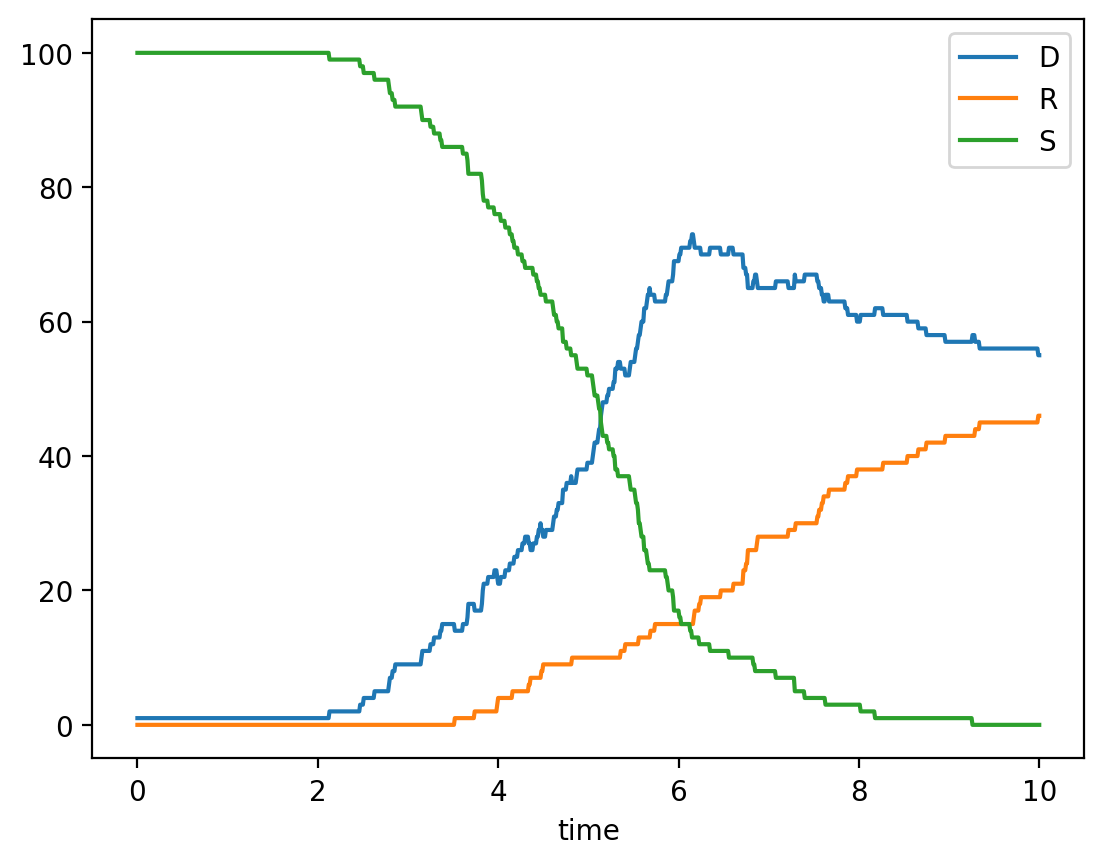
Unlike the regular Simulator.solve() which takes an iterable of times to save_at, RebopSimulator.solve() takes arguments upto_t to control simulation end time and n_points which decides how many equally spaced times are sampled. Since it doesn't count 0, n_points = N will a Dataset with a N + 1 size time coordinate:

len(result.coords["time"])
>>> 1001

To manually set a seed, we must pass it to the rng argument:

_result = rebsim.solve(n_points=1000, upto_t=10, rng=23534256).to_dataframe().plot()

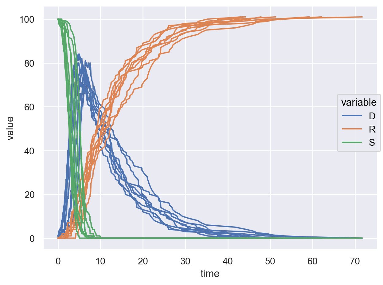
Of course, since the simulation is stochastic the result will be different every time its run. We can run it many times to get a better idea of the system's behaviour:

import seaborn.objects as so

df_100 = (
    xr.concat(
        [rebsim.solve(n_points=0, upto_t=100) for _ in range(10)],
        dim="seed",
        join="outer",
    )
    .to_dataframe()
    .melt(ignore_index=False)
    .reset_index()
)
df_100
so.Plot(df_100, x="time", y="value", color="variable", group="seed").add(so.Lines()).show()

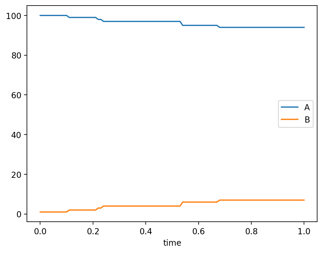
RateLaws and arbitrary rates

Stochastic simulation support a reduced subset of symbolite functions and operators for rates both in RateLaws and MassActions.

from symbolite import real
class Model(System):
    A: Variable = initial(default = 100)
    B: Variable = initial(default = 1)

    r = RateLaw(reactants = [A], products = [B], rate_law = real.sqrt(A)+1)
rebsim_2 = RebopSimulator(Model)
rebsim_2.solve(n_points=10, upto_t=1)

Rates and rate_laws can include:

• Basic operations: +, -, *, / and **.
• Functions that can be converted to powers: real.exp, real.sqrt and real.hypot.
• Functions that can be converted to multiplication: real.degrees and real.radians
• Mathematical constants: real.e, real.pi and real.tau.